Markov Process
Definition
- 元组 $(\mathcal{S,P})$
- $\mathcal{S}$是一个有限状态的集合
- $\mathcal{P}$是一个状态转移矩阵:$\mathcal{P_{ss’}}=\mathbb{P}[\mathcal{S_t+1}=s’|\mathcal{S_t}=s]$
Markov Reward Process
- 在前者的基础上,增加了$(\mathcal{S,P,\color{red}{\mathcal{R,\gamma}}})$
- $\color{red}{\mathcal{R}是一个奖励函数,\mathcal{R_s}=\mathbb{E}[R_{t+1}|\mathcal{S}=s]}$
- $\color{red}\gamma是一个衰减因子,\gamma\in[0,1]$
奖励函数$\mathcal{R}$代表了从状态$s$转移到状态$s’$时获得的奖励,这里奖励是离开状态后得到的(至于离开得到奖励还是进入一个新状态得到奖励只是定义了一种获得的规则而已)
$G_t$
代表了从状态$s$到最后状态$s_t$,得到的最终奖励,加入$\gamma$是因为距离越远,影响越小。即某一个具体 episode 所获得的 return。
目标是将其最大化。
价值函数(Value Function)
其代表着在状态$s$下的,$G_t$的期望值,因为从一个状态 s 出发有很多种不同的决策路径,得到不同的$G_t$
贝尔曼方程(Bellman equation)

最后一行理由为:x 的期望的期望是 x 期望其本身.得到了一个重要的递归公式:
其有两部分组成,及时奖励的期望$\boldsymbol{R_{t+1}}$ ,下一个时刻状态$\boldsymbol{s_{t+1}}$ 的期望
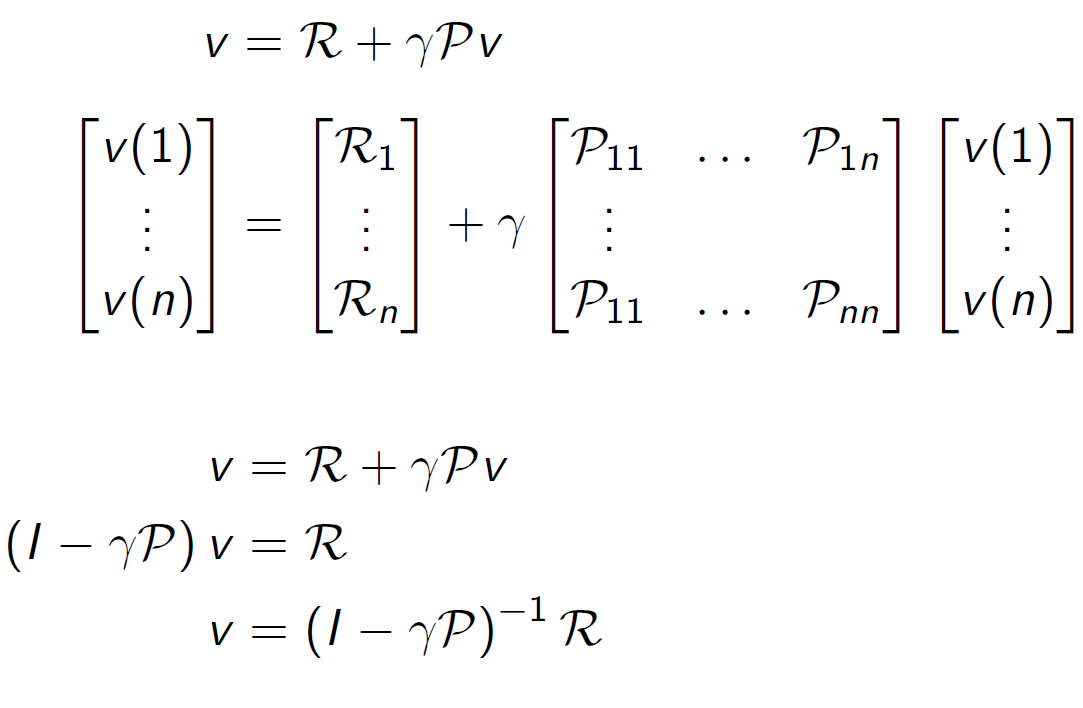
矩阵求解
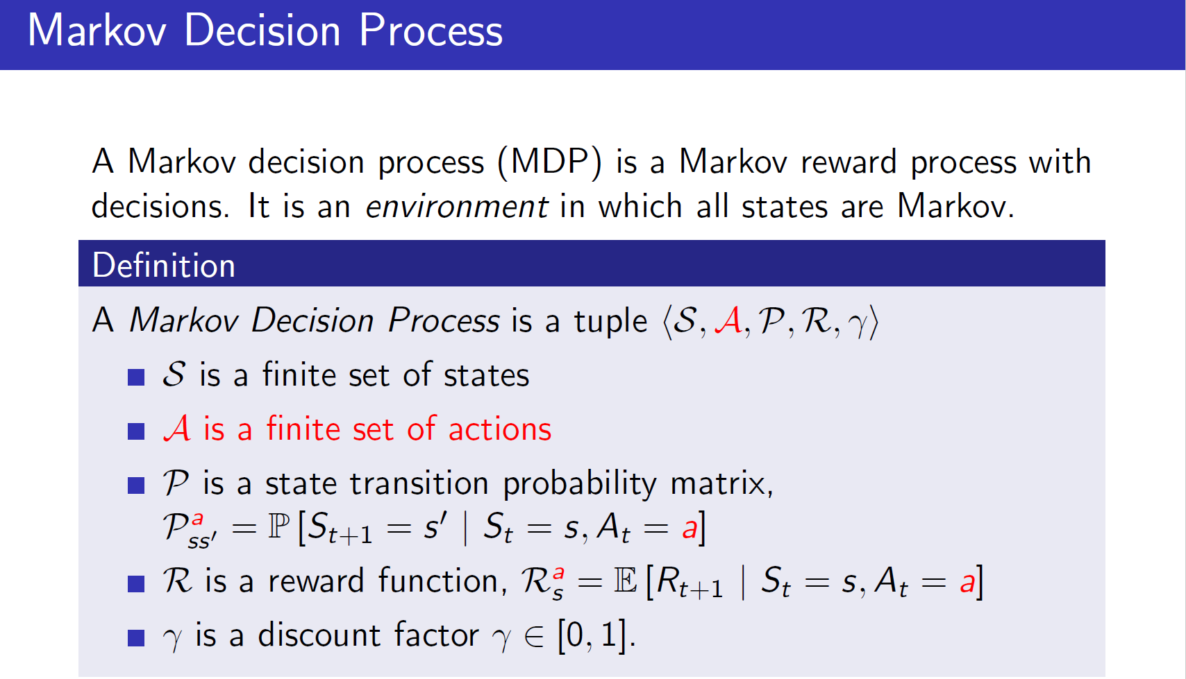
Markov Decision Process
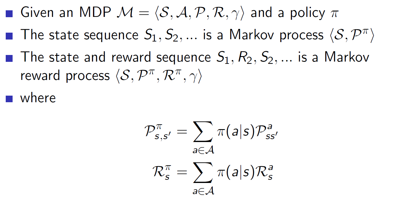
策略(policy)

策略代表了在给定状态$s$下,可能的动作概率分布。
价值函数-2

===>
可以发现,也是个递归地过程
$v_\pi(s)$是由当前状态$s$下,策略$\pi$可能的动作概率*该动作下得到的奖励值,累加而成
$q_\pi(s,a)$由两部分组成,及时回报和执行这个操作后可能到达所有状态$s’$的价值函数的累加
将其最优化
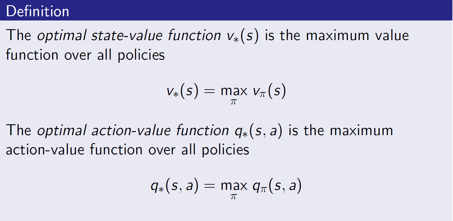
最优策略
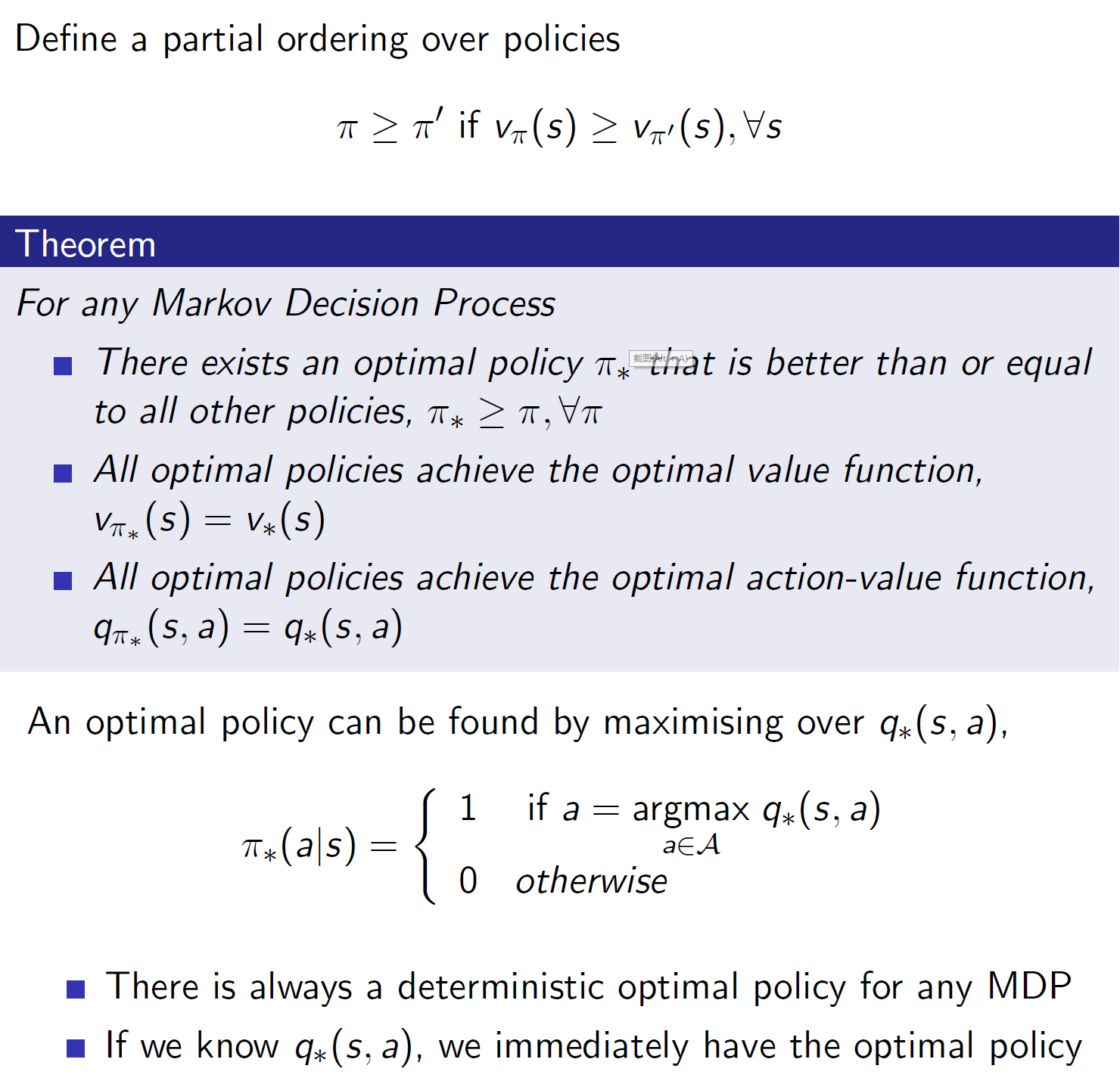
最优状态动作价值函数
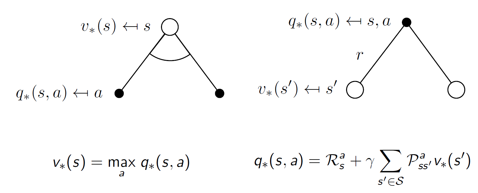
彼此带入:
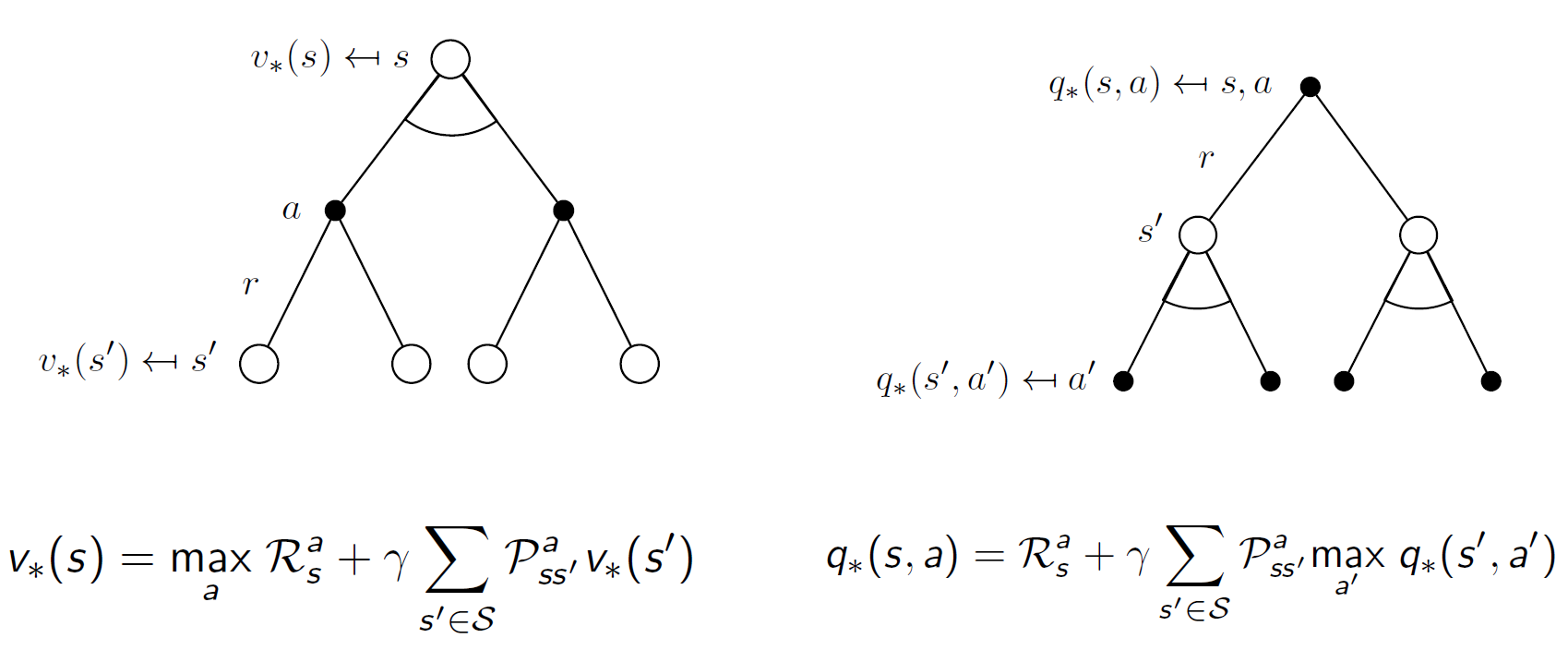
如何求解
得到最优解的递归形式,如何求解就很关键了。主要方法有:value Function(Q-learning,Sarsa);Policy gradient(PPO);AC 等等.
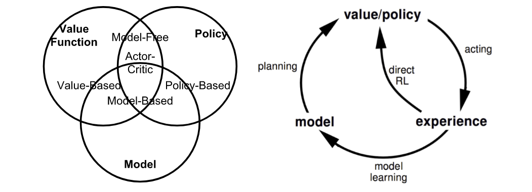
_Fig. Summary of approaches in RL based on whether we want to model the value, policy, or the environment. (Image source: reproduced from David Silver’s RL course lecture 1.)_
On-policy vs Off-policy
- Model-based: Rely on the model of the environment; either the model is known or the algorithm learns it explicitly.(_When we fully know the environment, we can find the optimal solution by Dynamic Programming (DP)._)
- Model-free: No dependency on the model during learning.
- Model-based尝试着 model 整个环境;先 model 了这个环境,基于该环境做出最优的策略;Model-free就是走一步看一步,在每一步中去尝试学习最优的策略。
_The model-based learning uses environment, action and reward to get the most reward from the action. The model-free learning only uses its action and reward to infer the best action._
On-policy: The agent learned and the agent interacting with the environment is the same.(自己和环境互动)
- Off-policy:The agent learned and the agent interacting with the environment is different.(自己看别人玩)
Policy
Policy $\pi$,代表在状态$s$,会执行的动作$a$.(分为确定性和随机性)
- Deterministic: $\pi(s)=a.$
- Stochastic: $\pi(a|s)=\mathbb{P}_\pi[A=a|S=s]$
- $\pi_\theta(a|s)=\mathbb{P}_\pi[A=a|S=s,\theta]$
Policy Gradient
object function:
episodic environments:
$J_1(\theta)=V^{\pi_\theta}(s_1)=\mathbb{E}_{\pi_\theta}[V_1]$
continuing environments:
_连续型环境就没有初始状态一说了,那么就取平均,考虑 agent 在某时刻处于某个状态下的概率,即状态分布_
average value:
$J_{avV}(\theta)=\sum_sd^{\pi_\theta}(s)V^{\pi_\theta}(s)$
对每个可能的状态计算从该时刻(该状态)开始于环境一直交互下去的奖励,然后对其概率分布求和.
average reward per time-step:
$J_{avR}(\theta)=\sum_sd^{\pi_\theta}(s)\sum_a\pi_\theta(s,a)\mathcal{R}_s^a$
其中,$d^{\pi_\theta}(s)$是马尔科夫链在$\pi_\theta$下的随机概率分布;即$d^\pi(s)=lim_{t→∞}P(s_t=s|s_0,\pi_θ)$就表示你从状态$s_0$开始,在策略$\pi_θ$下经过$t$个时间步后到达状态$s$的概率。
该式代表了到达某个状态$s$,并且采用动作$a$的情况下,获得的平均回报$\mathcal{R_s^a}$,概率化累加就是平均回报.
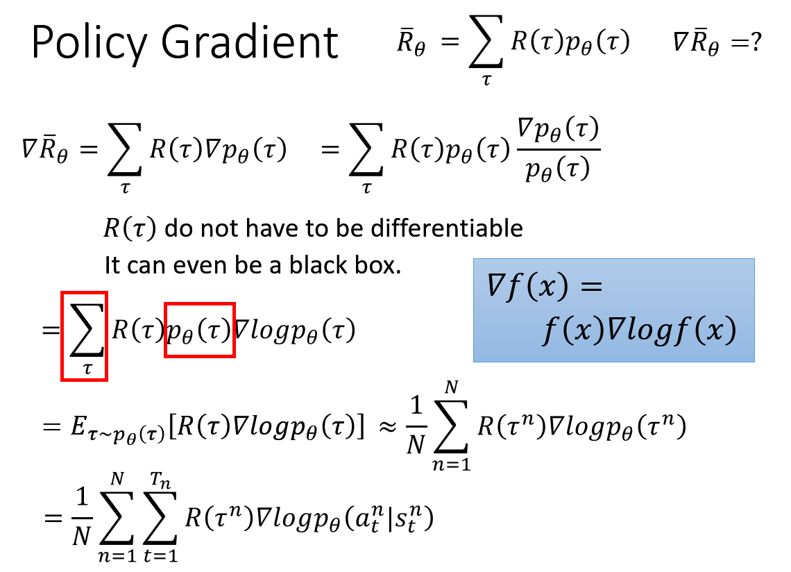
这个可以如下计算(以李宏毅教授 PPT 为例),每条迹的概率*该条迹累计的期望即为平均
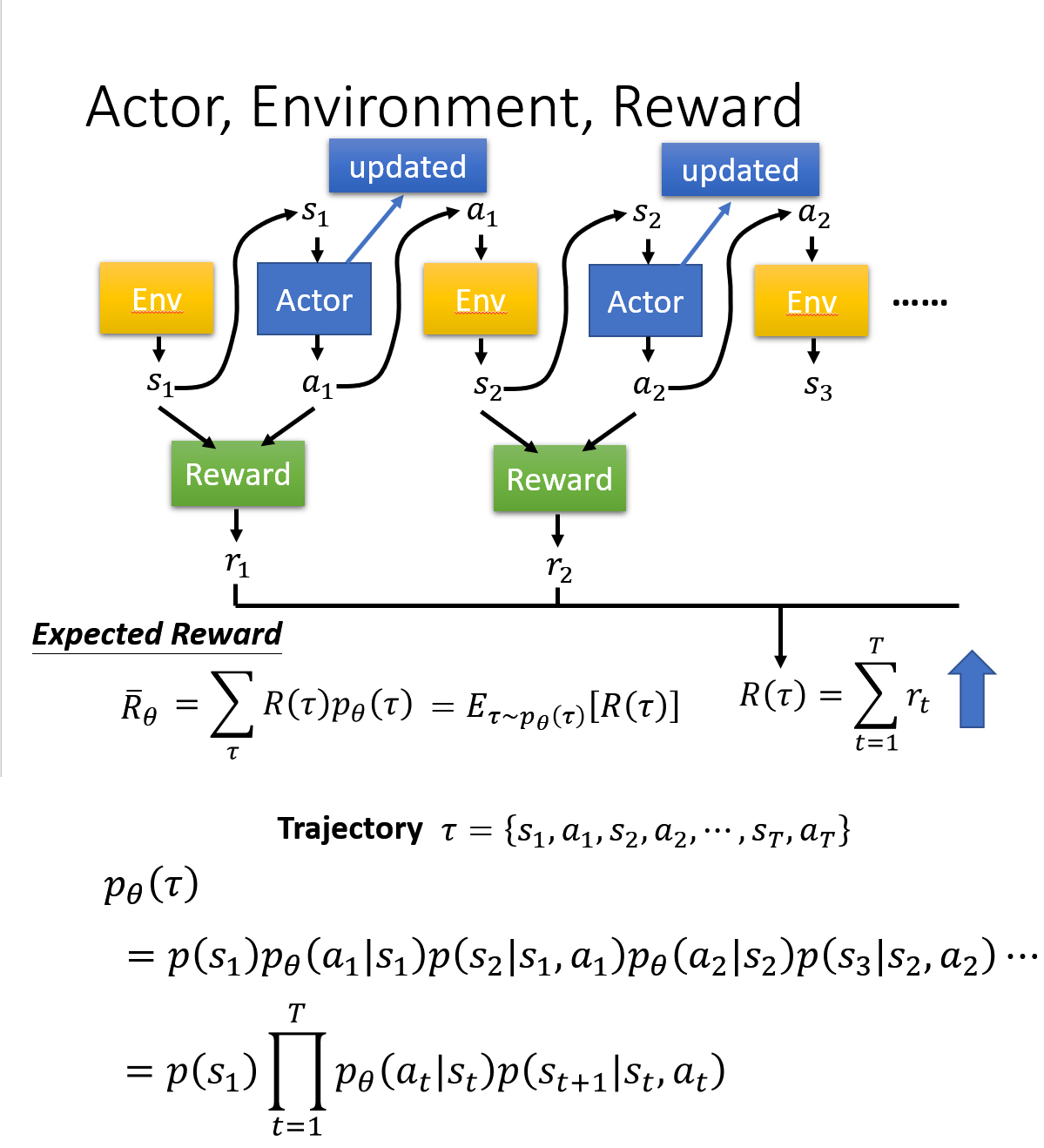
目标是将目标函数最大化,可以用梯度下降法将其最大化
_注:用基于梯度的策略优化时,是基于序列结构片段,如果无穷地和环境交互,得到一个结果是没有意义的;就是和环境交互中的某一个序列,将其拿出来进行学习,然后优化策略_
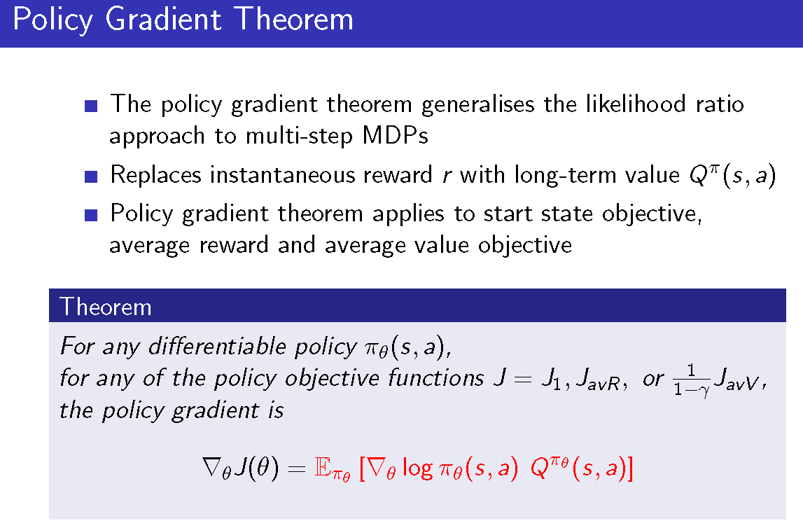
one-step MDP(per time-step):
==>policy gradient theorem
==>李宏毅教授 PPT
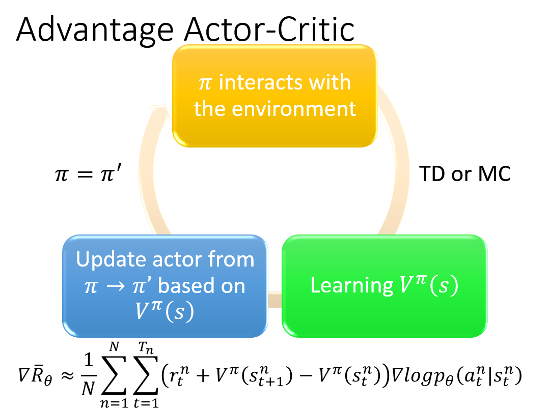
Actor-Critic
AC 是在基于 Policy Gradient 的基础上进行了变化,融合了 Value based 的方法.
Actor:就是把$J(\theta)$最大化,但是梯度里面的$Q^{\pi_\theta}(s,a)$用 Value based 的方法来计算,结果如下:
Reference
David Silver slides
博客:
https://lilianweng.github.io/lil-log/2018/04/08/policy-gradient-algorithms.html
李宏毅教授:
David_Silver:
配套 PPT
Mnih, Volodymyr, et al. “Asynchronous methods for deep reinforcement learning.” ICML. 2016.
David Silver, et al. “Deterministic policy gradient algorithms.” ICML. 2014.
Timothy P. Lillicrap, et al. “Continuous control with deep reinforcement learning.” arXiv preprint arXiv:1509.02971 (2015).
✉️ zexianchen@zju.edu.cn